Gamma Ray Spectroscopy Lab
PHYS 4410 - Advanced Physics Lab
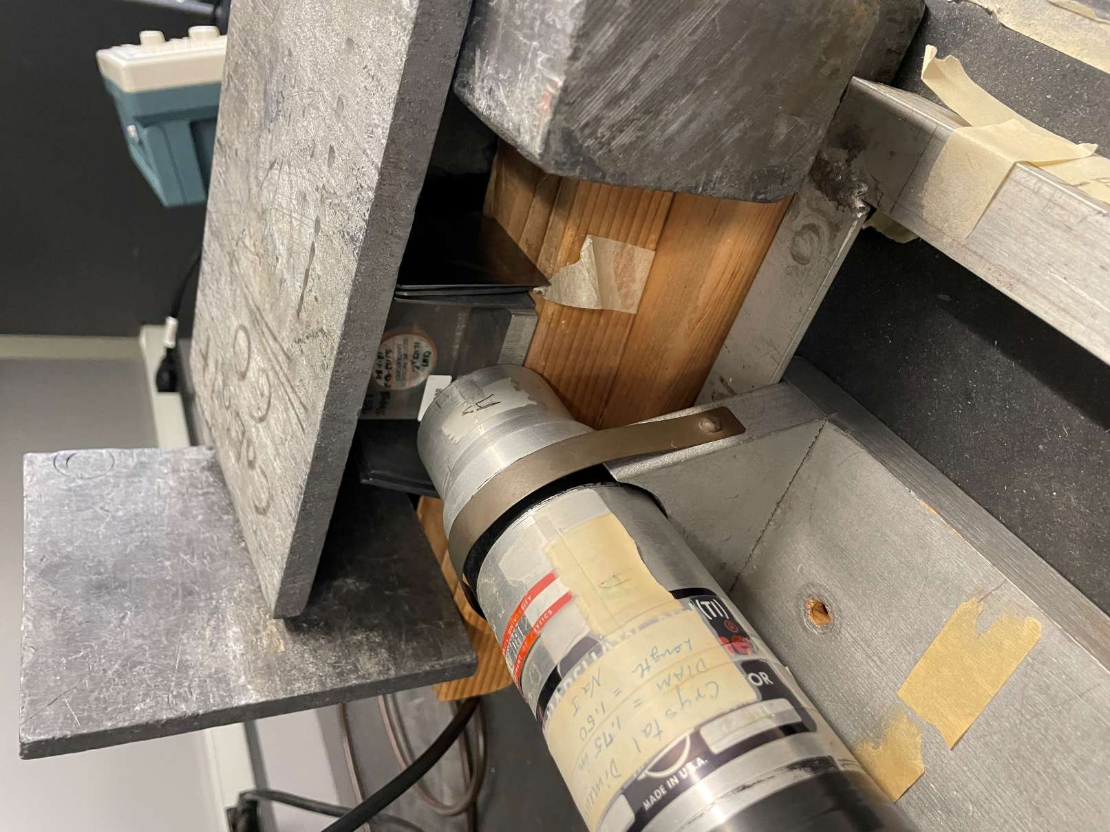
Since my research under LASSP involves gamma ray radiation, scintillation, and photomultiplier tubes (PMTs), I decided to spend my first lab in PHYS 4410 getting more familiar with these concepts by doing some Gamma Ray Spectroscopy. This lab is also particularly memorable for me because all of my data was originally taken on a modem running Windows XP, using amplifiers and other hardware that was out of the 70s and 80s. Even if the technology was ancient, it was able to give me great data and interesting findings in my report!
For each experimental trial, I would place my radiation source in the lead chamber, and record my results on the Pulse Height Analyzer (PHA) for around 30 minutes. The PHA would count the peak voltage measured by the PMT over short time intervals, and those voltages could be converted into the energy of the particle(s) that collided with the PMT. Since radioactive samples release very stable gamma radiation energies, the differences in these energies (when recorded over a long period of time) can be attributed to other physical processes, such as Compton Scattering, X-Ray photoabsorption, and the production of electron-positron pairs (antimatter!). I also ran a simulation of my experiment and compared the real results I observed to the Monte-Carlo results in an idealized setup.
In the end, I had some strange, unintuitive findings that surprised the professors running the course, but I think I was able to track down the cause of my findings to setting up the experiment differently than previous students. Specifically, I had used a thinner backing of tantalum in a lead-tantalum comparison test, which may have caused a backscatter rate to increase rather than decrease. The exact details are highlighted in my report, but they led me down an interesting “rabbit-hole” that allowed me to appreciate the complexity of solid-state physics, even for a relatively simple problem such as this one. This lab certainly helped me to better understand my lab work with Carl Franck, so I was happy I chose to do it first.
Torque Wrench
This project post is modified from a final assignment for MAE 3720 - Mechanics of Engineering Materials.
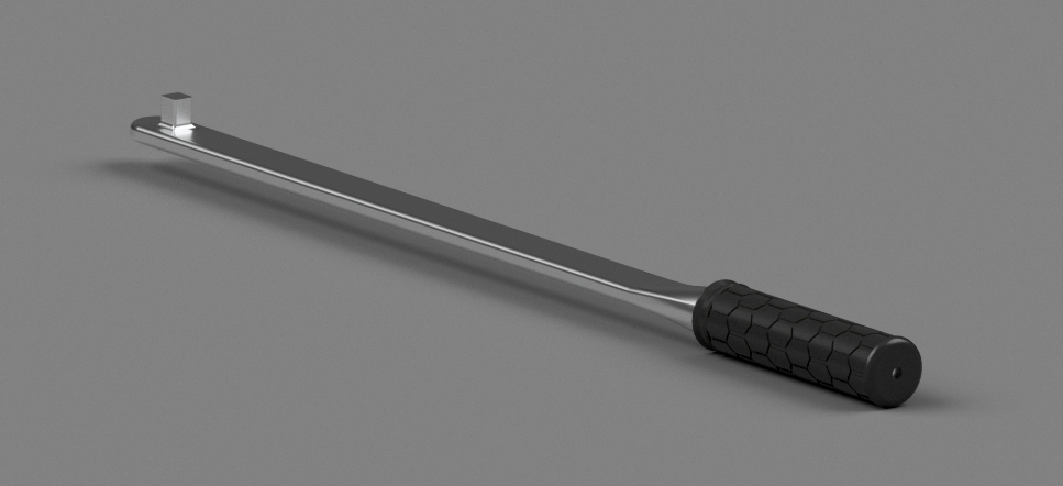
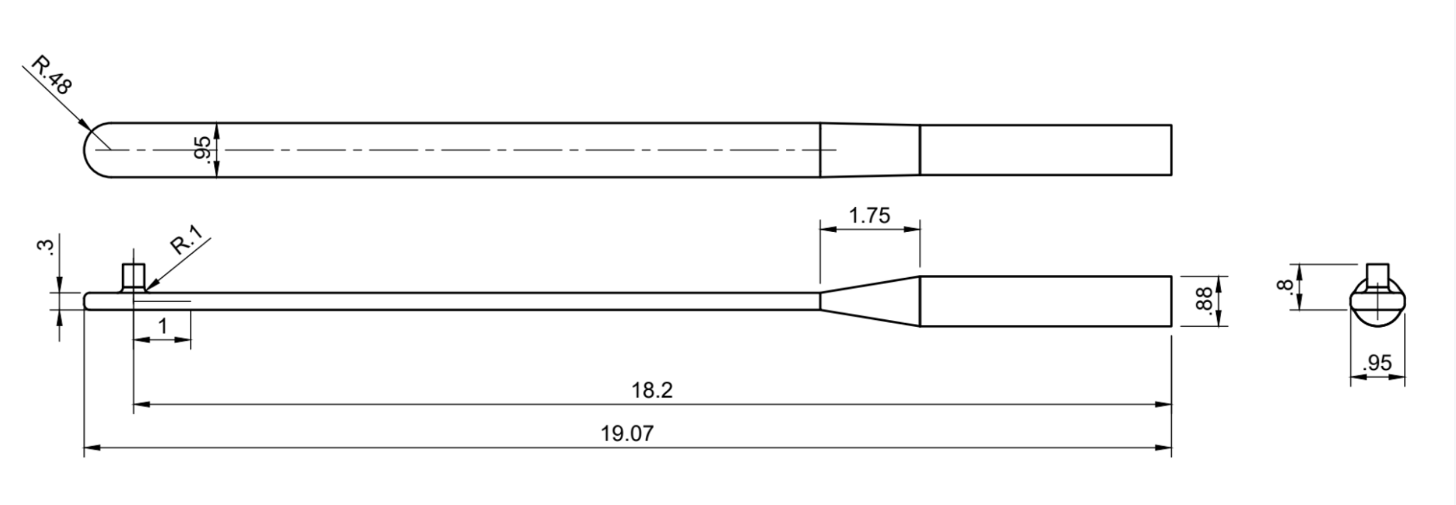
This is a render of our modified design of the torque wrench. It is made out of 7075-T6 aluminium, and has a rubber handle which makes it easier for a user to grip. The handle is circular, but transitions to a rectangular cross-section, similar to the baseline design. Key dimensions are shown in the drawing below (in inches). The cross-section of the rectangular portion of the wrench is 0.95” by 0.3”.
We are using 7075-T6 aluminum alloy for our final torque wrench design, which we landed on after comparing it to other aluminium, steel, and titanium options, as well as the original M42 tool steel (from the baseline design). The M42 had a much higher tensile strength than what was needed given the design constraints, so 7075-T6 aluminium (with a yield strength of 66.7 ksi) is a more reasonable option given its much cheaper cost (over 11 times cheaper). Other aluminium alloys, like 6061-T6 and 2024-T3, failed to be strong enough for the yield strength requirement without dramatically changing the overall dimensions. We also chose 7075-T6 over other steels (like AISI 1050 or 4140) for the lower elastic modulus, since these steels were only slightly cheaper in material cost but would require a more dramatic redesign of the overall dimensions to pass the strain gauge requirement. We also explored titanium options such as Grade 2 and Ti-6Al-4V, but these options were still many times more expensive than 7075-T6 even with changing the geometry to have a smaller overall cross-section/less volume.
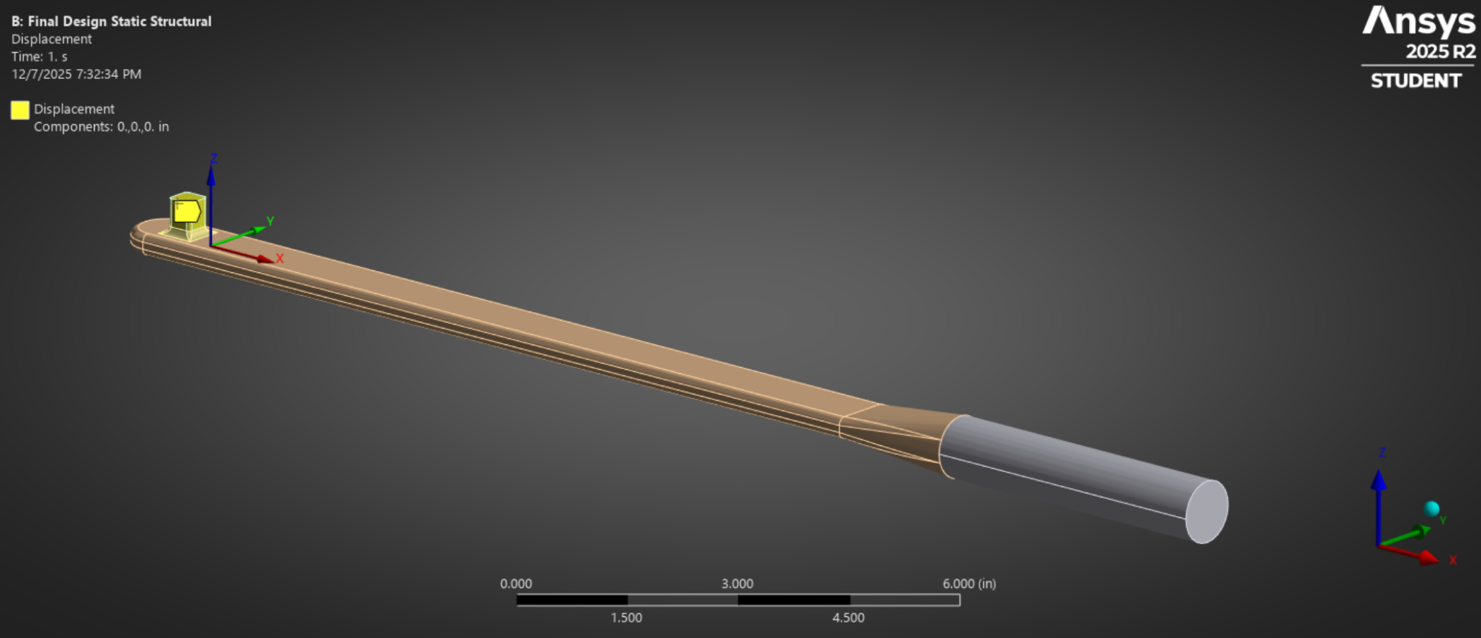
Our zero-displacement boundary condition remained unchanged between the baseline and final design. All five faces of the contact region at the end of the wrench are locked into place, with a 0.1” clearance given between this region and the rest of the wrench. A fillet connects the nub to the main body.
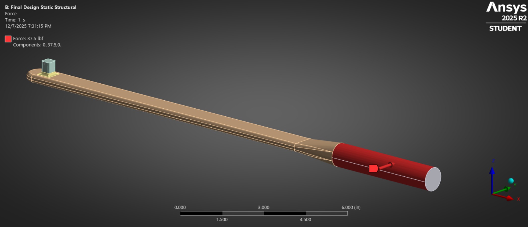
We did significantly change the force being applied at the end of the wrench, to more accurately reflect how the wrench is used. Since we added a large, rubber handle around the circular region of the wrench, we assume that the applied force is distributed evenly around the entire surface of the handle. To ensure the overall torque being applied is roughly the same as in the baseline case, we extended the wrench so the middle of the handle is at a distance of 16 inches from the fixed region.
To generate a mesh, we had to deviate significantly from the baseline case due to our loft geometry and the limitations of compute time for the student version of Ansys. Instead of Multizone, we switch to the automatic setting for mesh generation, since it, Hex, and other common meshes failed to generate between the loft and the cylinder. We also settled on the finest mesh we could, which was 0.2” for the main body of the wrench and handle, and 0.002” by the nub. We tested less-fine meshes prior to these settings, but larger body sizes for the nub led to even more pronounced stress concentrations.
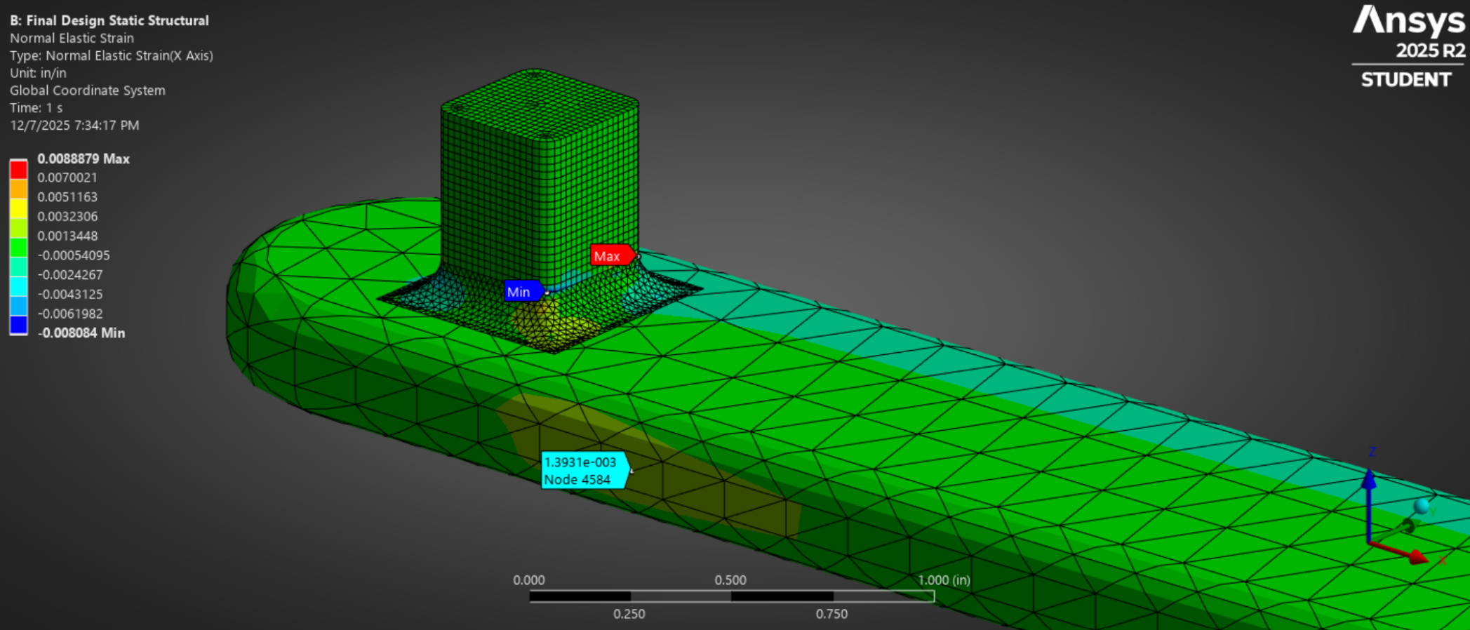
The normal strain contour plot shows that, at the same 1 inch spacing used for the strain gauge in the baseline wrench, our updated design has a strain of 1.3931e-3/
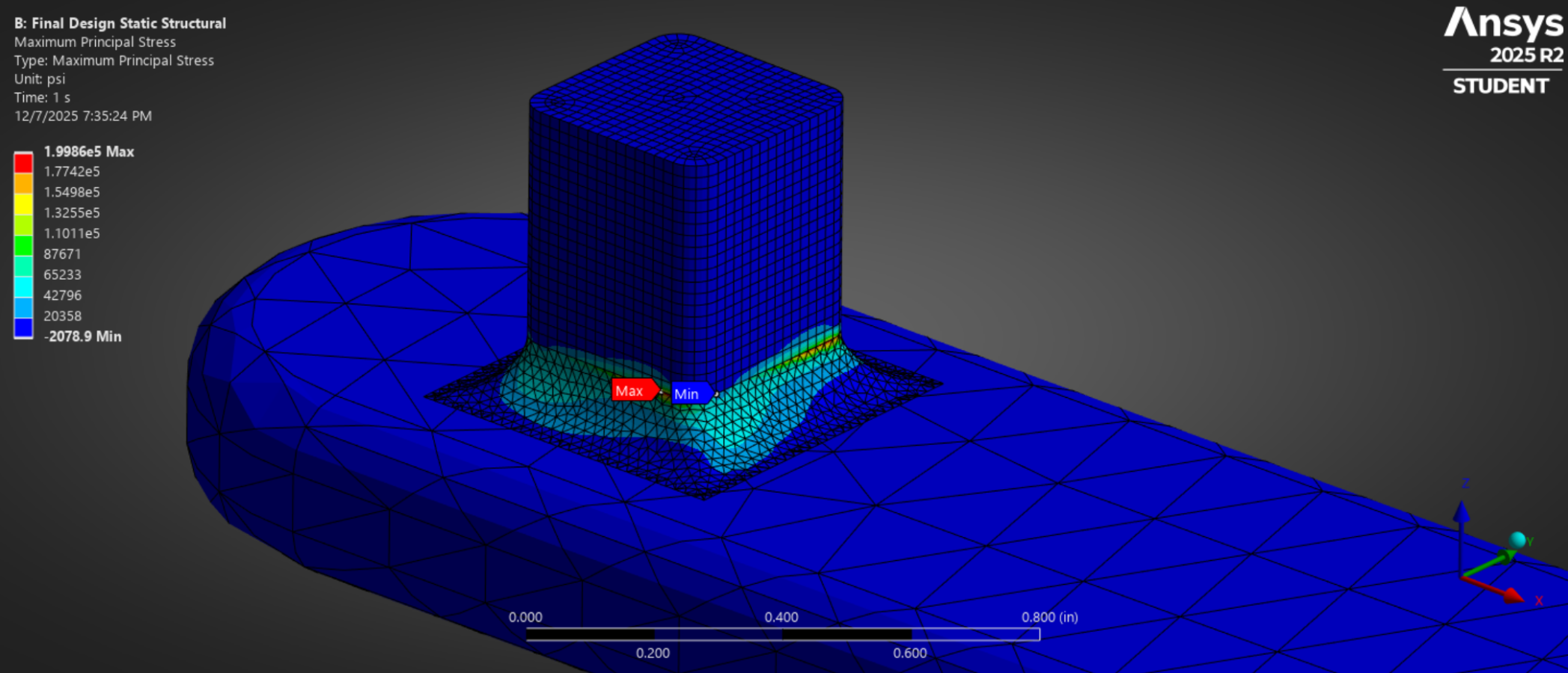
The principal stress contour plot shows how our boundary conditions are creating an artificial stress concentration. The maximum reported stress is 2.00e5 psi (200 ksi), which is much greater than our analytical hand calculations predict. However, the maximum normal stress just 1 node away from this maximum already drops down to 70.5 ksi, and disperses even more heavily from there. If we more accurately modeled the boundary conditions between the wrench and the part it slots into to turn, we would be able to more precisely determine the maximum principal stress.
Summarized Results:
Max Normal Stress (psi) - 2.00e5
Normal Stress 1 Node Removed from Max (psi) - 7.05e4
Load Point Deflection (in) - 0.437
Strain at Gauge Location - 1.393e-3
For our strain gauge, we have chosen a gauge with similar characteristics to the theoretical gauge used for the baseline model. We found the CEA-06-125UN-350 strain gauge (by Vishay Precision Group - Micro-Measurements), which is a half-bridge gauge with a gauge factor (k) of 2.1. This means our over torque wrench sensitivity is epsilon*k/2 = 1.463 mV/V. We also confirmed that the overall dimensions of the gauge (0.38” by 0.19”) fit on the side of our wrench and can be oriented properly (the short 0.19” side aligns with the 0.3” thickness of the wrench and fits snugly).
Cavendish Balance
PHYS 4410 - Advanced Physics Lab
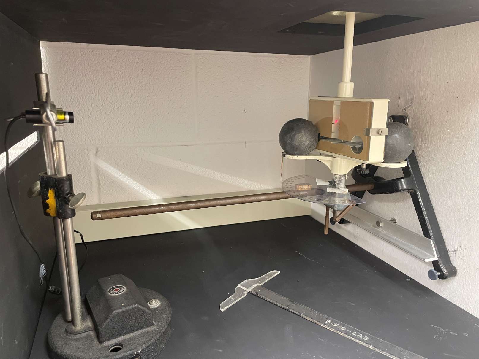
Of the three experiments I conducted in the advanced lab class, I think the Cavendish Balance was certainly the most fun. I was given a basic Cavendish balance apparatus, with the goal of extracting the gravitational constant G using a variety of set methods. I was given some key measurements about the apparatus (namely the dimensions of the dumbbell masses inside the box, since the apparatus was very delicate), but otherwise I needed to determine the most effective way to take data and properly model the system to the best of my ability. Since I wanted to get one method for measuring G that was especially accurate, I focused on curve-fitting the motion of the dumbbell to a damped sinusoidal.
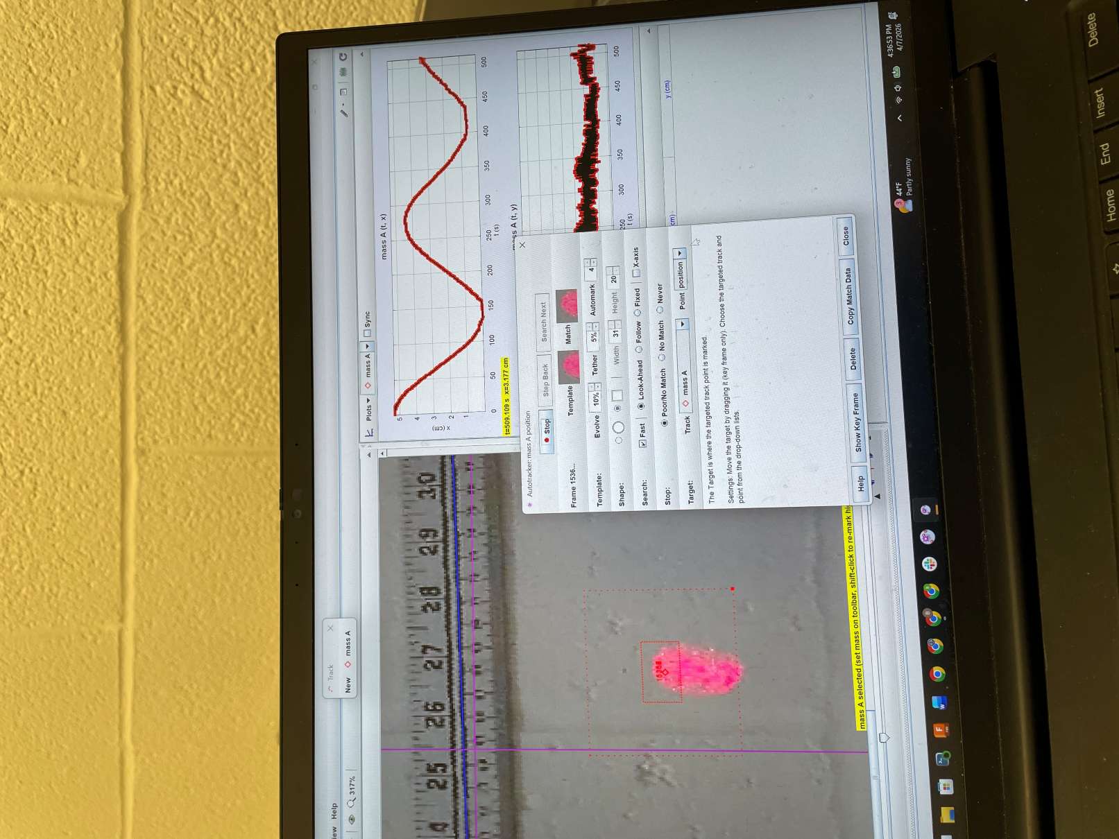
I had previously used the “Physics Tracker” software program before to track chromatic aberration in another class, so I figured that this program could help me track the motion of the laser dot which I recorded using the provided camera. When I initially assumed that the apparatus was aligned perfectly (propagating error for anything that was misaligned) and ran my curve fit, I found that I could measure G this way to about 25% accuracy. However, I was able to confirm with more careful inspection of the balance that components were significantly askew, which I documented in my report. Factoring these asymmetries more carefully, I was able to improve the accuracy of my measurement down to 6%, which was more precise than any students had recently obtained on my apparatus.
Since the Cavendish Balance is such a classic experiment, it was fun to see how I could actually obtain G within even an order of magnitude with such as simple setup. It was a nice way to end PHYS 4410!